List of electromagnetism equations

This article summarizes equations in the theory of electromagnetism.

DefinitionsEdit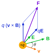

Lorentz force on a charged particle (of charge q) in motion (velocity v), used as the definition of the E field and B field.

Here subscripts e and m are used to differ between electric and magnetic charges. The definitions for monopoles are of theoretical interest, although real magnetic dipoles can be described using pole strengths. There are two possible units for monopole strength, Wb (Weber) and A m (Ampere metre). Dimensional analysis shows that magnetic charges relate by q_m(Wb) = μ₀ q_m(Am).

Initial quantitiesEdit

Quantity (common name/s)	(Common) symbol/s	SI units	Dimension
Electric charge	qe, q, Q	C = As	[I][T]
Monopole strength, magnetic charge	qm, g, p	Wb or Am	[L]2[M][T]−2 [I]−1 (Wb) [I][L] (Am)

Electric quantitiesEdit

Continuous charge distribution. The volume charge density ρ is the amount of charge per unit volume (cube), surface charge density σ is amount per unit surface area (circle) with outward unit normal n̂, d is the dipole moment between two point charges, the volume density of these is the polarization density P. Position vector r is a point to calculate the electric field; r′ is a point in the charged object.

Contrary to the strong analogy between (classical) gravitation and electrostatics, there are no "centre of charge" or "centre of electrostatic attraction" analogues.

Electric transport

Quantity (common name/s)	(Common) symbol/s	Defining equation	SI units	Dimension
Linear, surface, volumetric charge density	λe for Linear, σe for surface, ρe for volume.	${\displaystyle q_{e}=\int \lambda _{e}\mathrm {d} \ell }$ ${\displaystyle q_{e}=\iint \sigma _{e}\mathrm {d} S}$ ${\displaystyle q_{e}=\iiint \rho _{e}\mathrm {d} V}$	C m−n, n = 1, 2, 3	[I][T][L]−n
Capacitance	C	${\displaystyle C=\mathrm {d} q/\mathrm {d} V\,\!}$ V = voltage, not volume.	F = C V−1	[I]2[T]4[L]−2[M]−1
Electric current	I	${\displaystyle I=\mathrm {d} q/\mathrm {d} t\,\!}$	A	[I]
Electric current density	J	${\displaystyle I=\mathbf {J} \cdot \mathrm {d} \mathbf {S} }$	A m−2	[I][L]−2
Displacement current density	Jd	${\displaystyle \mathbf {J} _{\mathrm {d} }=\epsilon _{0}\left(\partial \mathbf {E} /\partial t\right)=\partial \mathbf {D} /\partial t\,\!}$	A m−2	[I][L]−2
Convection current density	Jc	${\displaystyle \mathbf {J} _{\mathrm {c} }=\rho \mathbf {v} \,\!}$	A m−2	[I][L]−2

Electric fields

Quantity (common name/s)	(Common) symbol/s	Defining equation	SI units	Dimension
Electric field, field strength, flux density, potential gradient	E	${\displaystyle \mathbf {E} =\mathbf {F} /q\,\!}$	N C−1 = V m−1	[M][L][T]−3[I]−1
Electric flux	ΦE	${\displaystyle \Phi _{E}=\int _{S}\mathbf {E} \cdot \mathrm {d} \mathbf {A} \,\!}$	N m2 C−1	[M][L]3[T]−3[I]−1
Absolute permittivity;	ε	${\displaystyle \epsilon =\epsilon _{r}\epsilon _{0}\,\!}$	F m−1	[I]2 [T]4 [M]−1 [L]−3
Electric dipole moment	p	${\displaystyle \mathbf {p} =q\mathbf {a} \,\!}$ a = charge separation directed from -ve to +ve charge	C m	[I][T][L]
Electric Polarization, polarization density	P	${\displaystyle \mathbf {P} =\mathrm {d} \langle \mathbf {p} \rangle /\mathrm {d} V\,\!}$	C m−2	[I][T][L]−2
Electric displacement field	D	${\displaystyle \mathbf {D} =\epsilon \mathbf {E} =\epsilon _{0}\mathbf {E} +\mathbf {P} \,}$	C m−2	[I][T][L]−2
Electric displacement flux	ΦD	${\displaystyle \Phi _{D}=\int _{S}\mathbf {D} \cdot \mathrm {d} \mathbf {A} \,\!}$	C	[I][T]
Absolute electric potential, EM scalar potential relative to point ${\displaystyle r_{0}\,\!}$ Theoretical: ${\displaystyle r_{0}=\infty \,\!}$ Practical: ${\displaystyle r_{0}=R_{\mathrm {earth} }\,\!}$ (Earth's radius)	φ ,V	${\displaystyle V=-{\frac {W_{\infty r}}{q}}=-{\frac {1}{q}}\int _{\infty }^{r}\mathbf {F} \cdot \mathrm {d} \mathbf {r} =-\int _{r_{1}}^{r_{2}}\mathbf {E} \cdot \mathrm {d} \mathbf {r} \,\!}$	V = J C−1	[M] [L]2 [T]−3 [I]−1
Voltage, Electric potential difference	Δφ,ΔV	${\displaystyle \Delta V=-{\frac {\Delta W}{q}}=-{\frac {1}{q}}\int _{r_{1}}^{r_{2}}\mathbf {F} \cdot \mathrm {d} \mathbf {r} =-\int _{r_{1}}^{r_{2}}\mathbf {E} \cdot \mathrm {d} \mathbf {r} \,\!}$	V = J C−1	[M] [L]2 [T]−3 [I]−1

Magnetic quantitiesEdit

Magnetic transport

Quantity (common name/s)	(Common) symbol/s	Defining equation	SI units	Dimension
Linear, surface, volumetric pole density	λm for Linear, σm for surface, ρm for volume.	${\displaystyle q_{m}=\int \lambda _{m}\mathrm {d} \ell }$ ${\displaystyle q_{m}=\iint \sigma _{m}\mathrm {d} S}$ ${\displaystyle q_{m}=\iiint \rho _{m}\mathrm {d} V}$	Wb m−n A m(−n + 1), n = 1, 2, 3	[L]2[M][T]−2 [I]−1 (Wb) [I][L] (Am)
Monopole current	Im	${\displaystyle I_{m}=\mathrm {d} q_{m}/\mathrm {d} t\,\!}$	Wb s−1 A m s−1	[L]2[M][T]−3 [I]−1 (Wb) [I][L][T]−1 (Am)
Monopole current density	Jm	${\displaystyle I=\iint \mathbf {J} _{\mathrm {m} }\cdot \mathrm {d} \mathbf {A} }$	Wb s−1 m−2 A m−1 s−1	[M][T]−3 [I]−1 (Wb) [I][L]−1[T]−1 (Am)

Magnetic fields

Quantity (common name/s)	(Common) symbol/s	Defining equation	SI units	Dimension
Magnetic field, field strength, flux density, induction field	B	${\displaystyle \mathbf {F} =q_{e}\left(\mathbf {v} \times \mathbf {B} \right)\,\!}$	T = N A−1 m−1 = Wb m−2	[M][T]−2[I]−1
Magnetic potential, EM vector potential	A	${\displaystyle \mathbf {B} =\nabla \times \mathbf {A} }$	T m = N A−1 = Wb m3	[M][L][T]−2[I]−1
Magnetic flux	ΦB	${\displaystyle \Phi _{B}=\int _{S}\mathbf {B} \cdot \mathrm {d} \mathbf {A} \,\!}$	Wb = T m2	[L]2[M][T]−2[I]−1
Magnetic permeability	${\displaystyle \mu \,\!}$	${\displaystyle \mu \ =\mu _{r}\,\mu _{0}\,\!}$	V·s·A−1·m−1 = N·A−2 = T·m·A−1 = Wb·A−1·m−1	[M][L][T]−2[I]−2
Magnetic moment, magnetic dipole moment	m, μB, Π	Two definitions are possible: using pole strengths, ${\displaystyle \mathbf {m} =q_{m}\mathbf {a} \,\!}$ using currents: ${\displaystyle \mathbf {m} =NIA\mathbf {\hat {n}} \,\!}$ a = pole separation N is the number of turns of conductor	A m2	[I][L]2
Magnetization	M	${\displaystyle \mathbf {M} =\mathrm {d} \langle \mathbf {m} \rangle /\mathrm {d} V\,\!}$	A m−1	[I] [L]−1
Magnetic field intensity, (AKA field strength)	H	Two definitions are possible: most common: ${\displaystyle \mathbf {B} =\mu \mathbf {H} =\mu _{0}\left(\mathbf {H} +\mathbf {M} \right)\,}$ using pole strengths,[1] ${\displaystyle \mathbf {H} =\mathbf {F} /q_{m}\,}$	A m−1	[I] [L]−1
Intensity of magnetization, magnetic polarization	I, J	${\displaystyle \mathbf {I} =\mu \mathbf {M} \,\!}$	T = N A−1 m−1 = Wb m−2	[M][T]−2[I]−1
Self Inductance	L	Two equivalent definitions are possible: ${\displaystyle L=N\left(\mathrm {d} \Phi /\mathrm {d} I\right)\,\!}$ ${\displaystyle L\left(\mathrm {d} I/\mathrm {d} t\right)=-NV\,\!}$	H = Wb A−1	[L]2 [M] [T]−2 [I]−2
Mutual inductance	M	Again two equivalent definitions are possible: ${\displaystyle M_{1}=N\left(\mathrm {d} \Phi _{2}/\mathrm {d} I_{1}\right)\,\!}$ ${\displaystyle M\left(\mathrm {d} I_{2}/\mathrm {d} t\right)=-NV_{1}\,\!}$ 1,2 subscripts refer to two conductors/inductors mutually inducing voltage/ linking magnetic flux through each other. They can be interchanged for the required conductor/inductor; ${\displaystyle M_{2}=N\left(\mathrm {d} \Phi _{1}/\mathrm {d} I_{2}\right)\,\!}$ ${\displaystyle M\left(\mathrm {d} I_{1}/\mathrm {d} t\right)=-NV_{2}\,\!}$	H = Wb A−1	[L]2 [M] [T]−2 [I]−2
Gyromagnetic ratio (for charged particles in a magnetic field)	γ	${\displaystyle \omega =\gamma B\,\!}$	Hz T−1	[M]−1[T][I]

Electric circuitsEdit

DC circuits, general definitions

Main article: Direct current

Quantity (common name/s)	(Common) symbol/s	Defining equation	SI units	Dimension
Terminal Voltage for Power Supply	Vter		V = J C−1	[M] [L]2 [T]−3 [I]−1
Load Voltage for Circuit	Vload		V = J C−1	[M] [L]2 [T]−3 [I]−1
Internal resistance of power supply	Rint	${\displaystyle R_{\mathrm {int} }=V_{\mathrm {ter} }/I\,\!}$	Ω = V A−1 = J s C−2	[M][L]2 [T]−3 [I]−2
Load resistance of circuit	Rext	${\displaystyle R_{\mathrm {ext} }=V_{\mathrm {load} }/I\,\!}$	Ω = V A−1 = J s C−2	[M][L]2 [T]−3 [I]−2
Electromotive force (emf), voltage across entire circuit including power supply, external components and conductors	E	${\displaystyle {\mathcal {E}}=V_{\mathrm {ter} }+V_{\mathrm {load} }\,\!}$	V = J C−1	[M] [L]2 [T]−3 [I]−1

AC circuits

Main articles: Alternating current and Resonance

Quantity (common name/s)	(Common) symbol/s	Defining equation	SI units	Dimension
Resistive load voltage	VR	${\displaystyle V_{R}=I_{R}R\,\!}$	V = J C−1	[M] [L]2 [T]−3 [I]−1
Capacitive load voltage	VC	${\displaystyle V_{C}=I_{C}X_{C}\,\!}$	V = J C−1	[M] [L]2 [T]−3 [I]−1
Inductive load voltage	VL	${\displaystyle V_{L}=I_{L}X_{L}\,\!}$	V = J C−1	[M] [L]2 [T]−3 [I]−1
Capacitive reactance	XC	${\displaystyle X_{C}={\frac {1}{\omega _{\mathrm {d} }C}}\,\!}$	Ω−1 m−1	[I]2 [T]3 [M]−2 [L]−2
Inductive reactance	XL	${\displaystyle X_{L}=\omega _{d}L\,\!}$	Ω−1 m−1	[I]2 [T]3 [M]−2 [L]−2
AC electrical impedance	Z	${\displaystyle V=IZ\,\!}$ ${\displaystyle Z={\sqrt {R^{2}+\left(X_{L}-X_{C}\right)^{2}}}\,\!}$	Ω−1 m−1	[I]2 [T]3 [M]−2 [L]−2
Phase constant	δ, φ	${\displaystyle \tan \phi ={\frac {X_{L}-X_{C}}{R}}\,\!}$	dimensionless	dimensionless
AC peak current	I0	${\displaystyle I_{0}=I_{\mathrm {rms} }{\sqrt {2}}\,\!}$	A	[I]
AC root mean square current	Irms	${\displaystyle I_{\mathrm {rms} }={\sqrt {{\frac {1}{T}}\int _{0}^{T}\left[I\left(t\right)\right]^{2}\mathrm {d} t}}\,\!}$	A	[I]
AC peak voltage	V0	${\displaystyle V_{0}=V_{\mathrm {rms} }{\sqrt {2}}\,\!}$	V = J C−1	[M] [L]2 [T]−3 [I]−1
AC root mean square voltage	Vrms	${\displaystyle V_{\mathrm {rms} }={\sqrt {{\frac {1}{T}}\int _{0}^{T}\left[V\left(t\right)\right]^{2}\mathrm {d} t}}\,\!}$	V = J C−1	[M] [L]2 [T]−3 [I]−1
AC emf, root mean square	${\displaystyle {\mathcal {E}}_{\mathrm {rms} },{\sqrt {\langle {\mathcal {E}}\rangle }}\,\!}$	${\displaystyle {\mathcal {E}}_{\mathrm {rms} }={\mathcal {E}}_{\mathrm {m} }/{\sqrt {2}}\,\!}$	V = J C−1	[M] [L]2 [T]−3 [I]−1
AC average power	${\displaystyle \langle P\rangle \,\!}$	${\displaystyle \langle P\rangle ={\mathcal {E}}I_{\mathrm {rms} }\cos \phi \,\!}$	W = J s−1	[M] [L]2 [T]−3
Capacitive time constant	τC	${\displaystyle \tau _{C}=RC\,\!}$	s	[T]
Inductive time constant	τL	${\displaystyle \tau _{L}=L/R\,\!}$	s	[T]

Magnetic circuitsEdit

Main article: Magnetic circuits

Quantity (common name/s)	(Common) symbol/s	Defining equation	SI units	Dimension
Magnetomotive force, mmf	F, ${\displaystyle {\mathcal {F}},{\mathcal {M}}}$	${\displaystyle {\mathcal {M}}=NI}$ N = number of turns of conductor	A	[I]

ElectromagnetismEdit

Electric fieldsEdit

General Classical Equations

Physical situation	Equations
Electric potential gradient and field	${\displaystyle \mathbf {E} =-\nabla V}$ ${\displaystyle \Delta V=-\int _{r_{1}}^{r_{2}}\mathbf {E} \cdot d\mathbf {r} \,\!}$
Point charge	${\displaystyle \mathbf {E} ={\frac {q}{4\pi \epsilon _{0}\left|\mathbf {r} \right|^{2}}}\mathbf {\hat {r}} \,\!}$
At a point in a local array of point charges	${\displaystyle \mathbf {E} =\sum \mathbf {E} _{i}={\frac {1}{4\pi \epsilon _{0}}}\sum _{i}{\frac {q_{i}}{\left|\mathbf {r} _{i}-\mathbf {r} \right|^{2}}}\mathbf {\hat {r}} _{i}\,\!}$
At a point due to a continuum of charge	${\displaystyle \mathbf {E} ={\frac {1}{4\pi \epsilon _{0}}}\int _{V}{\frac {\mathbf {r} \rho \mathrm {d} V}{\left|\mathbf {r} \right|^{3}}}\,\!}$
Electrostatic torque and potential energy due to non-uniform fields and dipole moments	${\displaystyle {\boldsymbol {\tau }}=\int _{V}\mathrm {d} \mathbf {p} \times \mathbf {E} }$ ${\displaystyle U=\int _{V}\mathrm {d} \mathbf {p} \cdot \mathbf {E} }$

Magnetic fields and momentsEdit

See also: Magnetic moment

General classical equations

Physical situation	Equations
Magnetic potential, EM vector potential	${\displaystyle \mathbf {B} =\nabla \times \mathbf {A} }$
Due to a magnetic moment	${\displaystyle \mathbf {A} ={\frac {\mu _{0}}{4\pi }}{\frac {\mathbf {m} \times \mathbf {r} }{\left|\mathbf {r} \right|^{3}}}}$ ${\displaystyle \mathbf {B} ({\mathbf {r} })=\nabla \times {\mathbf {A} }={\frac {\mu _{0}}{4\pi }}\left({\frac {3\mathbf {r} (\mathbf {m} \cdot \mathbf {r} )}{\left|\mathbf {r} \right|^{5}}}-{\frac {\mathbf {m} }{\left|\mathbf {r} \right|^{3}}}\right)}$
Magnetic moment due to a current distribution	${\displaystyle \mathbf {m} ={\frac {1}{2}}\int _{V}\mathbf {r} \times \mathbf {J} \mathrm {d} V}$
Magnetostatic torque and potential energy due to non-uniform fields and dipole moments	${\displaystyle {\boldsymbol {\tau }}=\int _{V}\mathrm {d} \mathbf {m} \times \mathbf {B} }$ ${\displaystyle U=\int _{V}\mathrm {d} \mathbf {m} \cdot \mathbf {B} }$

Electric circuits and electronicsEdit

Below N = number of conductors or circuit components. Subcript net refers to the equivalent and resultant property value.

Physical situation	Nomenclature	Series	Parallel
Resistors and conductors	Ri = resistance of resistor or conductor i Gi = conductance of resistor or conductor i	${\displaystyle R_{\mathrm {net} }=\sum _{i=1}^{N}R_{i}\,\!}$ ${\displaystyle {1 \over G_{\mathrm {net} }}=\sum _{i=1}^{N}{1 \over G_{i}}\,\!}$	${\displaystyle {1 \over R_{\mathrm {net} }}=\sum _{i=1}^{N}{1 \over R_{i}}\,\!}$ ${\displaystyle G_{\mathrm {net} }=\sum _{i=1}^{N}G_{i}\,\!}$
Charge, capacitors, currents	Ci = capacitance of capacitor i qi = charge of charge carrier i	${\displaystyle q_{\mathrm {net} }=\sum _{i=1}^{N}q_{i}\,\!}$ ${\displaystyle {1 \over C_{\mathrm {net} }}=\sum _{i=1}^{N}{1 \over C_{i}}\,\!}$ ${\displaystyle I_{\mathrm {net} }=I_{i}\,\!}$	${\displaystyle q_{\mathrm {net} }=\sum _{i=1}^{N}q_{i}\,\!}$ ${\displaystyle C_{\mathrm {net} }=\sum _{i=1}^{N}C_{i}\,\!}$ ${\displaystyle I_{\mathrm {net} }=\sum _{i=1}^{N}I_{i}\,\!}$
Inductors	Li = self-inductance of inductor i Lij = self-inductance element ij of L matrix Mij = mutual inductance between inductors i and j	${\displaystyle L_{\mathrm {net} }=\sum _{i=1}^{N}L_{i}\,\!}$	${\displaystyle {1 \over L_{\mathrm {net} }}=\sum _{i=1}^{N}{1 \over L_{i}}\,\!}$ ${\displaystyle V_{i}=\sum _{j=1}^{N}L_{ij}{\frac {\mathrm {d} I_{j}}{\mathrm {d} t}}\,\!}$

Series circuit equations

Circuit	DC Circuit equations	AC Circuit equations
RC circuits	Circuit equation ${\displaystyle R{\frac {\mathrm {d} q}{\mathrm {d} t}}+{\frac {q}{C}}={\mathcal {E}}\,\!}$ Capacitor charge ${\displaystyle q=C{\mathcal {E}}\left(1-e^{-t/RC}\right)\,\!}$ Capacitor discharge ${\displaystyle q=C{\mathcal {E}}e^{-t/RC}\,\!}$
RL circuits	Circuit equation ${\displaystyle L{\frac {\mathrm {d} I}{\mathrm {d} t}}+RI={\mathcal {E}}\,\!}$ Inductor current rise ${\displaystyle I={\frac {\mathcal {E}}{R}}\left(1-e^{-Rt/L}\right)\,\!}$ Inductor current fall ${\displaystyle I={\frac {\mathcal {E}}{R}}e^{-t/\tau _{L}}=I_{0}e^{-Rt/L}\,\!}$
LC circuits	Circuit equation ${\displaystyle L{\frac {\mathrm {d} ^{2}q}{\mathrm {d} t^{2}}}+q/C={\mathcal {E}}\,\!}$	Circuit equation ${\displaystyle L{\frac {\mathrm {d} ^{2}q}{\mathrm {d} t^{2}}}+q/C={\mathcal {E}}\sin \left(\omega _{0}t+\phi \right)\,\!}$ Circuit resonant frequency ${\displaystyle \omega _{\mathrm {res} }=1/{\sqrt {LC}}\,\!}$ Circuit charge ${\displaystyle q=q_{0}\cos(\omega t+\phi )\,\!}$  Circuit current ${\displaystyle I=-\omega q_{0}\sin(\omega t+\phi )\,\!}$  Circuit electrical potential energy ${\displaystyle U_{E}=q^{2}/2C=Q^{2}\cos ^{2}(\omega t+\phi )/2C\,\!}$ Circuit magnetic potential energy ${\displaystyle U_{B}=Q^{2}\sin ^{2}(\omega t+\phi )/2C\,\!}$
RLC Circuits	Circuit equation ${\displaystyle L{\frac {\mathrm {d} ^{2}q}{\mathrm {d} t^{2}}}+R{\frac {\mathrm {d} q}{\mathrm {d} t}}+{\frac {q}{C}}={\mathcal {E}}\,\!}$	Circuit equation ${\displaystyle L{\frac {\mathrm {d} ^{2}q}{\mathrm {d} t^{2}}}+R{\frac {\mathrm {d} q}{\mathrm {d} t}}+{\frac {q}{C}}={\mathcal {E}}\sin \left(\omega _{0}t+\phi \right)\,\!}$ Circuit charge ${\displaystyle q=q_{0}eT^{-Rt/2L}\cos(\omega 't+\phi )\,\!}$

This article uses material from the Wikipedia article  Metasyntactic variable, which is released under the  Creative Commons Attribution-ShareAlike 3.0 Unported License.